BIO315 Laboratory Guide #7
ACOUSTICAL ANALYSIS OF BIRDSONG
USING RAVENTM
A primary mode of animal communication is by sounds. This laboratory will familiarize you with some of the methodologies and analytical tools for bioacoustical analysis of animal calls. The centerpiece of this lab will be a computer application called Raven , developed by the Cornell Ornithological Laboratory.
Bioacoustical analysis begins with a recording of an animal sound. The Macauley Library at Cornell University is a library of digital recordings of animal calls, available for downloading. The Cornell Laboratory of Ornithology also produces a CD of representative songs from all of the known birds in North America, and we will use this for a reference.
Prior to this lab period you have practiced techniques for recording animal calls in the wild, including the use of directional microphones. Raven has tools for transferring these "raw" recordings to computer files, "cleaning" the recordings by filtering out unwanted sounds, amplifying the sounds, and playing the sounds back through the computer speakers. Because many animal sounds either fall below or above the range of human auditory discrimination (e.g. whale calls and frog calls, respectively) Raven can slow or speed up the calls on playback. Raven can also be used for constructing novel call sequences by splicing together fragments from existing calls.
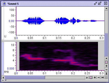
As you can imagine, humans are much better at visual analysis than at auditory analysis. The real power of the Raven application is its ability to produce several standard types of visual representations of sounds. The simplest of these is a waveform plot, as shown in the top trace of the example above. In this plot, the X axis represents time, while the Y axis represents sound pressure. An easy way to understand what this plot shows is to think of it as a running time plot of the movement of an imaginary speaker face which is producing the sound. In the plot above, the blue line is tracing the "sound envelope" - basically the loudness of the sound as it waxes and wanes during the call. As the X axis is expanded, the actual waveform of the sound can be seen in the form of individual vibrations.
An alternative way to display the properties of an entire sound sample is to plot frequency on the X axis and power on the Y axis. This produces a plot called a spectrogram. The power at each frequency is determined by converting the entire complex waveform into an equivalent set of simple sine waves, using a mathematical tool called Fourier analysis. The spectrogram is then produced by plotting the relative amplitude of each of the component sine waves against its frequency.
In the spectrogram, much of the timing or temporal resolution is lost - the spectrogram represents a collapsed time period. One method that captures the frequency vs. power analysis of the spectrogram and the temporal resolution of the waveform plot is a sonogram, as depicted in the lower trace above. In a sonogram, a simplified version of Fourier analysis, called the fast Fourier Transform (FFT) is used to produce a power spectrum for successive very short time intervals. These are then plotted with the X axis depicting the passage of time and the Y axis depicting sound frequency (pitch), expressed in Hz (cycles/second). Sound pressure or power (loudness) is represented by the density of the plot at each point. This may be plotted as a simple grey scale darkness, or as a false color spectrum, as in the example above.
I. LEARNING HOW TO USE THE RAVEN SOFTWARE
FOR BIOACOUSTICAL ANALYSIS
A. Finding and Opening Raven
1) Locate the Raven 1.2 folder on the desktop.
2) Open it and click on the Raven bird icon associated with the RavenLauncher application. This will open Raven 1.2.
B. Display, Playback, and Temporal Editing of a Prerecorded Song
1) Using the Open Sound Files Command in the File menu, find and open the file called "loon". You will find this file in the Canary Transfer folder, which is probably on the desktop.
2) When the file opens you should see two plots. The upper plot is a blue "waveform plot" display of the call of a common loon. The lower plot is a sonogram, such as you have already seen in your text. For now, deselect the sonogram plot by unchecking Spectrograph 1 near the top of the control panel at the left of the display.
3) To play back the loon call, click on the triangular arrow icon in the command bar. Adjust the speakers to a tolerable loudness and play the call again. Notice that as the call is played a green line moves across the waveform display, indicating what part of the call is being played at each moment in time. If you left click anywhere in the display window, Raven assumes that you are establishing a “selection” for special attention or analysis and sets a red marker at that location. This can interfere with subsequent playback and get pretty frustrating. To clear out the red marks, right click anywhere in the display window and then click on Clear All Selections.
4) A waveform plot graphs sound pressure as a function of time. Think of the plot as a graph of how the face of a loudspeaker would move as the song was being played. At this time resolution all you see is the “envelope” of the waveform.
5) Zoom the X-axis (time scale) of the waveform plot using the “+” zoom button at the bottom of the display. As you zoom you will have to use the horizontal slider to keep an interesting part of the call centered in the display. Continue to zoom until you can see individual waves of sound.
Q1: Why might this extreme temporal resolution be useful?
Q2: Does rescaling the visual display affect the auditory playback?
6) Continue to zoom until you see the individual data points displayed. In order to digitally represent a signal without significantly distorting it the digital sampling rate must be at least twice as high as the highest oscillation frequency of the signal. Dezoom back to the original horizontal scale using the “–“ button or by simply clicking on the bracket button to the right of the “-“ button.
7) Pull down the Edit menu, select Amplify, and choose an amplification factor of 2.0.
Q3: Does this affect both the visual display and the audio output?
8) Amplify again and again and again (16x total). Notice that the signal is now “clipped” – the extremes of sound pressure have been clipped off and flattened and the playback sounds distorted. Use the pull-down Edit menu to repeatedly deamplify the signal back to its original appearance.
9) Try adjusting the speed of the playback by entering a rate other than 1.0 in the Rate box at the upper right of the display window. Notice that as the rate slows down the pitch drops.
Q4: Why does the pitch drop as you slow down the playback rate?
Q5: Why might you slow down or speed up an animal sound in order to better understand it?
10) IMPORTANT - DO NOT SAVE CHANGES TO ANY OF THESE LIBRARY FILES. Open some of the other files of animal sounds. These may be found in the Canary Transfer folder on the desktop and or in the Examples folder. Notice that you don’t have to close old files in order to open new ones: Raven can keep multiple files open simultaneously. Try to find the best playback speed for analyzing each sound using just your ears.
11) Finally, notice that you can select a portion of a waveform plot by clicking and dragging over it. Experiment with cutting and pasting segments of a song to rearrange it using the standard Windows edit commands (Control x, c, and v for cut, copy, and paste, respectively). Make sure that you do NOT save the altered song when you are finished.
C. Sonogram Plots
A spectrogram tells you something about what sound frequencies make up each part of your recording, and how high the relative amplitude (loudness) of each frequency is at each point in time. Spectrograms of animal calls are generally called "sonograms".
1) Open the canada warbler file in Canary Transfer. Play the recording once to hear what the song sounds like.
2) Now eliminate the existing sonogram plot by clicking anywhere in the sonogram plot, pulling down the View menu and clicking on Delete View.
3) There are five icons at the upper left under the pull-down menus. Produce a new sonogram by clicking on the middle icon which looks like three horizontal gray bars. In the dialog box, leave all of the settings at their default values and click on OK. The new sonogram will be labeled Spectrogram 2 (because you just eliminated Spectrogram 1).
4) Try adjusting the Brightness and Contrast sliders at the top of the display window, until the sonogram plot shows the clearest detail. Note: to activate these sliders you will have to first select the Spectrogram by clicking anywhere in the spectrogram part of the display. If you click in the vertical box at the right of the sonogram you can activate that portion of the window without invoking the annoying red “selection” lines and boxes.
The sonogram plots time on the horizontal axis, just as the waveform plot does. The vertical axis of the sonogram shows frequency (pitch) at each moment of the song. Darkness of the sonogram plot shows the relative amplitude (loudness) of each frequency component.
5) Raven offers three alternative intensity scales to the grayscale you have been looking at so far. You can try out the other three scales by pulling down the View menu, selecting Color Scheme and choosing Hot, Cool, or Standard Gamma II. Experiment with the Brightness and Contrast sliders for each of these color schemes. Personally, I find these hard to interpret, but they look cool
6) Play the Canada Warbler song again. Notice that as the cursor tracks across the waveform plot it also tracks across the sonogram. Try to follow and predict the changes in pitch of the song from the sonogran, i.e. try to read it the way you might read a musical score. IF you can't do this successfully, try slowing the song to a rate of 0.3.
D. Producing a Power Spectrum (FFT Analysis)
1) Now open the w meadowlark file in the Canary Transfer folder. Play the sample once to see what it sounds like. Adjust Brightness and Contrast to get a good-looking sonogram.
2) Go up to the row of five icons at the upper left and choose the icon with the three vertical red bars. When the dialog box opens just click on OK. This opens a third display window which displays one of two disappointing phrases “There is currently no active selection” or “The active selection is too short to compute a spectrum”.
The Fourier transform is based on the fact that any sound, no matter how complex, can be broken down in the "frequency domain" into a unique set of sine waves. Each sine wave component has a unique frequency, amplitude, and phase. The FFT approximates this in a fast analysis (hence fast Fourier transform).
3) To perform a fast Fourier transform (FFT) on any section of the song, just click and drag in either the waveform or spectrogram windows. Notice that the new Spectrum window has different axes. The X axis is now frequency and the Y axis is a logarithmic amplitude (power) scale. In fact, a sonogram is produced by taking a sequence of spectrums from successive very short time-slices of the original signal, standing the spectrums on end, side-by-side, and gluing them back together.
4) Select the first phrase of the meadowlark song by clicking, dragging and releasing. This will calculate the power spectrum for just the selected part of the song. Notice that this first phrase is really a single extended note with a single dominant frequency of just under 4 kHz. Play this selection to confirm this with your ears. A rate of about .5 works well.
5) Select the second phrase in the song. Does the dominant frequency go up or down? Does this agree with what you hear and what the sonogram shows?
6) Select each successive phrase in turn and observe the power spectrum for each. Do the later phrases show more complex power spectra?
7) Click and drag to select the descending trill one second into the meadowlark song. Play this at several speeds. It is hard to believe this complex sound is coming out of the syrynx or voice box of a single bird.
E. Visually Identifying an Unknown Sound Source
1) Open the files called w meadowlark, canada warbler, rs towhee, whippoorwill, unkn 1, and unkn 2. You should now have six pairs of waveform/sonogram traces on your screen.
2) Each of the unknowns (unkn’s) is a fragment from one of the four bird songs. Your task is to match each unknown to the appropriate song.
3) Hints:
a) You might start by organizing your traces, so that you can find
them all
b) You might also think about rescaling the horizontal axis on each,
so that all of the traces have the same time scale.
4) Close all files when you are finished. IMPORTANT - DO NOT SAVE CHANGES TO THESE FILES.
II. THE ACTUAL LABORATORY EXERCISE AND WRITEUP
Complete the following three analyses. Illustrate your report with printed copies of Raven display windows. When printing, choose “Best” quality.
A. Analysis of Song Phrases in the Black-Capped Vireo
1) Open the BlackCappedVireo file in the Examples folder. Play the song. It is, needless to say, complex. Adjust the Contrast and Brightness of the sonogram. Hit the horizontal zoom at least five times to stretch out the song into distinct phrases. Slow the playback rate down to .2 or so. Open a Spectrum window.
2) Use the standard Windows cut and paste commands to rearrange the song so that similar looking and sounding phrases are clustered together. How many distinct “words” are there in the Black Capped Vireo song? (If you get a number less than 25 you are not trying hard enough).
3) Report on this analysis and any other aspects of the Black Capped Vireo song which you find interesting.
B. Analysis of Call Phrases in the Northern Cricket Frog
1) Open the n cricket frog file in the Canary Transfer folder.
2) Play it.
3) Notice that the call consists of a series of click complexes. Each click complex consists of some number of actual clicks. Perform and report on an analysis of this call, addressing the following questions, and any others you find interesting:
a) How does the timing of the click complexes evolve through the call?
Does each complex consist of the same number of clicks? If not, what?
Does the pause between complexes stay the same length? If not, what?
b) How similar are individual clicks within each complex, in terms of frequency, length, amplitude? How similar are individual clicks between complexes?
c) Does each click have a single, dominant frequency? How "clean" is each click (nearly sinusoidal or broad band/multiple frequency)?
d) Given that the sound-generating apparatus of the cricket frog consists not of a vibrating vocal cord, but of "pops" generated by air forced out of a vocal sac in the floor of the vocal cavity, do your results make sense?
C. Dialects of Effete Liberal Northern and Born-Again Redneck Southern Blue Jays
1) Open the bluejay CLO and jay comp WC files in the Canary Transfer folder. The first of these files is from a CD of bird songs from the Cornell Lab of Ornithology and was recorded under nearly ideal conditions from a jay in New Jersey (“nuh joy-zee”). The second file was recorded by your instructor from a jay on the Wesleyan campus in Georgia (“joh-juh”) under less than ideal field conditions. This second file has been digitally filtered to reduce background noise.
2) Play both files.
3) Notice that the recording of each jay consists of a two rather distinct types of call - a raucous "jay" call, and a more melodic "twitter".
4) Use everything that you have learned to characterize, compare, and contrast the call components of Jersey and Georgia Jays in an analysis and report on your analysis. A good way to do this would be use the cut and paste and Amplify functions to create one or more composite files with the "jay" call from the two birds right next to each other and the "twitter" call of the two birds right next to each other. Address the following questions and any others you find interesting:
a) Notice from the sonogram that the "jay" call is a neatly stacked set of harmonics (integer multiples of a base frequency). Verify this with a power spectrum. Is there anything peculiar about these stacks? For instance, what is the base frequency and how strongly is it represented? What is the strongest harmonic?
b) Are the Jersey and Georgia crows doing the "jay" call at the same pitch? Does what you see in the sonogram and power spectrum agree with what you hear?
c) How, specifically do the "twitter" calls of the two birds differ? Are they, for example, composed of the same parts, but simply produced in a different order?
III . ALTERNATIVE LAB EXERCISES
You may substitute the either of the following sets for ALL of the above three analyses. The instructor will help you do this.
A) Songbird
1) Record a bird song or call from the Wesleyan Arboretum using a directional microphone and digitial recorder.
2) Perform a tentative identification of the bird, either in the field, by listening to the recording, or by playing the recording to Dr. Ferrari.
3) Transfer the recording to a Raven-compatible AIFF file.
4) Transfer a corresponding “standard” call or song from the CLO CD of Eastern US bird songs.
5) Using Raven waveform, spectrogram, and spectrum analysis verify the species identity of your sample bird. Include appropriate Raven plots in your writeup.
6) Briefly discuss any differences between your field-recorded call/song and the CLO standard.
~OR~
B) Mockingbird
1) Record a mockingbird song from the Wesleyan Arboretum using a directional microphone and digital recorder.
2) Perform a tentative identification of the bird species which the mockingbird is mimicking, either in the field, by listening to the recording, or by playing the recording to Dr. Ferrari.
3) Transfer the recording to a Raven-compatible AIFF file.
4) Transfer a corresponding “standard” call or song for the mimicked bird from the CLO CD of Eastern US bird songs.
5) Using Raven waveform, spectrogram, and spectrum analysis verify the match between your mockingbird recording and the mimicked bird song. Include appropriate Raven plots in your writeup.
6) Briefly discuss any differences between the target bird song and the mockingbird version.